TL;DR
- AUROC is a ranking probability. It’s the chance that the model scores a randomly chosen positive case above a randomly chosen negative case. An AUROC of 0.75 gets that pair right three times out of four. Mathematically, it’s the Mann–Whitney U statistic rescaled to 0–1.
- AUROC doesn’t change with prevalence or with any rescaling of the scores. That makes it good for comparing ranking ability, and blind to three things you usually care about:
- how well the model does at the top of the list, where a team with finite capacity actually works;
- whether the scores are real probabilities;
- whether acting on the model does more good than harm.
- In the experiments below, two models with identical AUROC (0.75) differ by a factor of 1.8 in precision on their top 1%. Distorting a model’s probabilities leaves AUROC at 0.780 while the calibration slope falls from 0.98 to 0.49.
- What to report: AUROC with a confidence interval, PR-AUC next to its prevalence baseline, precision@k at real capacity, a calibration plot, and a decision curve. Break all of them down by subgroup.
“So, is 0.75 good?”
Picture the end of a model review. The data scientist puts up the final slide: “AUROC 0.75”. There’s a pause, and then the service manager asks the only question that matters to them:
“So if my team phones the twenty patients your model picks each week, how many of them would actually have missed their appointment?”
AUROC can’t answer that question. Neither can accuracy, F1 or most of the numbers that end up on the last slide. They aren’t wrong; they answer different questions. The skill is knowing which number answers which question, and which questions no single number can answer.
“A metric is an answer. Before you quote it, make sure you know the question.”
While writing up two case studies on predicting missed outpatient appointments, I kept using shorthand like “AUROC 0.77”, “PR-AUC against a 0.10 baseline” and “precision@20”. This post unpacks that vocabulary properly, from definitions to the statistics underneath, and tests each claim with an experiment you can rerun. The examples are about missed hospital appointments (“Did Not Attend”, or DNA), but the ideas apply to any binary risk model: fraud, churn, readmission, credit default.
The experiments use simulated data with a fixed random seed. Each one states its set-up (model, prevalence, sample size) next to the results, so you can rebuild it in a few lines of scikit-learn.
Contents
- Scores are not decisions
- A ten-patient worked example
- The confusion matrix and why accuracy misleads
- AUROC in depth: definition, statistics, properties and uncertainty
- Precision–recall and the prevalence baseline
- Precision@k: the metric for teams with finite capacity
- Calibration: can you read the score as a probability?
- Net benefit: is the model worth using at all?
- Beyond AUROC: more metrics worth knowing
- What to report, and common traps
- Three questions before you trust a risk model
1. Scores are not decisions
A risk model outputs a score for each case, usually between 0 and 1. For example, “Patient A: 0.82, Patient B: 0.07”. A score becomes a decision only when you add:
- a threshold (“flag everyone at or above 0.5”), or
- a capacity (“call the 20 highest-scoring patients this week”).
Think of a popular restaurant on a Friday night. The score is the queue outside, ordered by how likely each guest is to want a table. The threshold or capacity is the rope at the door: “seats for twenty”. Some metrics judge how well the queue is ordered. Others judge who actually got through the rope. They are different questions.
That splits evaluation metrics into two families:
| Family | Judges | Examples |
|---|---|---|
| Threshold-free | the scores themselves | AUROC, PR-AUC, calibration, Brier score |
| Threshold- or capacity-dependent | the decision made with the scores | accuracy, precision, recall, F1, precision@k, net benefit |
Most confusion about metrics comes from quoting one family to answer a question that belongs to the other.
2. A ten-patient worked example
Ten appointments, sorted by score. Three were actually missed:
| Rank | Score | Missed? |
|---|---|---|
| 1 | 0.90 | ✅ |
| 2 | 0.80 | — |
| 3 | 0.60 | ✅ |
| 4 | 0.50 | — |
| 5 | 0.40 | — |
| 6 | 0.30 | ✅ |
| 7 | 0.20 | — |
| 8 | 0.15 | — |
| 9 | 0.10 | — |
| 10 | 0.05 | — |
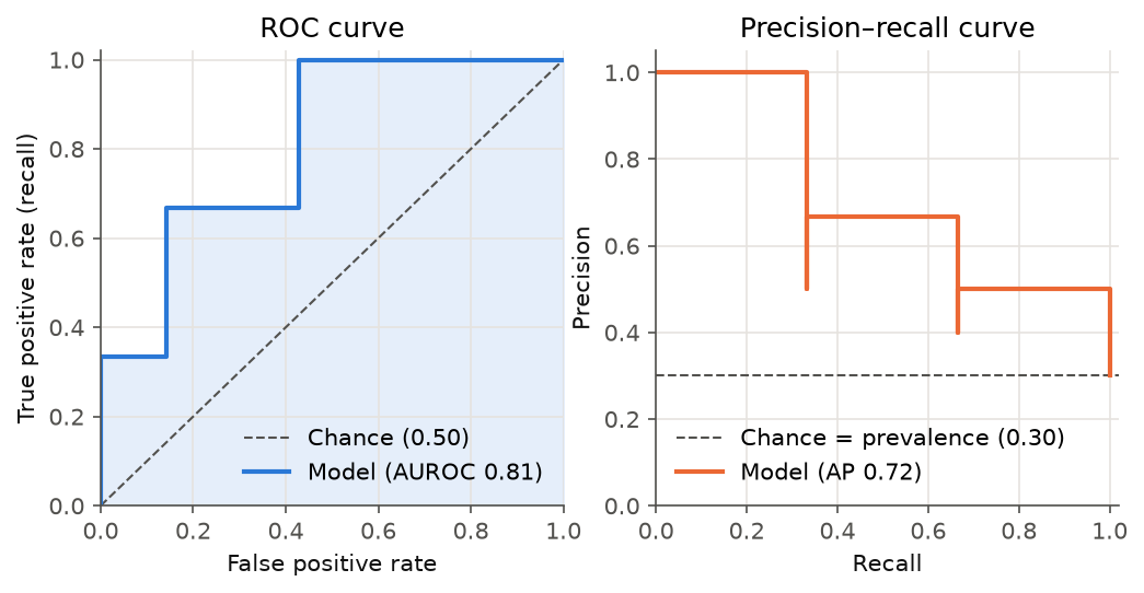
Figure 1. ROC and precision–recall curves for the worked example. Each upward or leftward step is one patient crossing the threshold as it falls.
3. The confusion matrix and why accuracy misleads
Set a threshold of 0.5. Ranks 1–4 are predicted “will miss”:
| Predicted miss | Predicted attend | |
|---|---|---|
| Actually missed | TP = 2 | FN = 1 |
| Actually attended | FP = 2 | TN = 5 |
| Metric | Formula | Question it answers | Here |
|---|---|---|---|
| Accuracy | (TP + TN) / N | How often is the model right? | 0.70 |
| Precision (PPV) | TP / (TP + FP) | Of those flagged, how many missed? | 0.50 |
| Recall (sensitivity, TPR) | TP / (TP + FN) | Of those who missed, how many were flagged? | 0.67 |
| Specificity (TNR) | TN / (TN + FP) | Of those who attended, how many were left alone? | 0.71 |
| False positive rate (FPR) | FP / (FP + TN) | Of those who attended, how many were flagged? | 0.29 |
| F1 | 2 · P · R / (P + R) | A balance of precision and recall | 0.57 |
Recall and specificity are conditioned on the true class, so they don’t depend on prevalence. Precision is conditioned on the predicted class, so it does. That one fact explains most of what follows.
Why accuracy misleads on rare outcomes. In my hackathon DNA model, 8.8% of appointments were missed. A Random Forest reached 91% accuracy, which is exactly what “everyone attends” scores. Its recall for missed appointments was 0.6% (37 of 6,612). A logistic regression with balanced class weights managed only 56% accuracy, but recall of 60%, at a precision of 12%. These two models aren’t “more” and “less” accurate. They’re different trade-offs, and accuracy hides both.
4. AUROC in depth
4.1 The ROC curve
Sweep the threshold from +∞ down to −∞. At each step, plot the TPR (y) against the FPR (x).
- A perfect model rises straight to (0, 1): it catches every positive before raising a single false alarm.
- A random model follows the diagonal.
- The name “receiver operating characteristic” comes from Second World War radar engineering, where operators traded detecting aircraft against false alarms.
4.2 What the area actually means
The area under that curve has an exact probabilistic meaning (Hanley & McNeil, 1982):
AUROC = P(score of a random positive > score of a random negative), counting ties as ½.
An analogy: a round-robin tournament. Put every patient who missed in one team and every patient who attended in the other. Each player from the first team plays a head-to-head match against every player from the second, and the higher score wins. AUROC is the first team’s win rate. It says nothing about by how much they won, or about which matches you’ll actually watch. Keep that in mind; it explains every limitation below.
Check it by hand on the worked example. There are 3 positives × 7 negatives = 21 pairs:
- The positive at 0.90 outranks all 7 negatives.
- The positive at 0.60 outranks 6 (it loses only to 0.80).
- The positive at 0.30 outranks 4.
(7 + 6 + 4) / 21 = 17 / 21 = 0.81.
That pair count is exactly the Mann–Whitney U statistic. So AUROC = U / (n₊ · n₋), which is why AUROC is also called the concordance statistic (c-statistic). Three implementations agree:
import numpy as np
from scipy.stats import mannwhitneyu
from sklearn.metrics import roc_auc_score

y = np.array([1, 0, 1, 0, 0, 1, 0, 0, 0, 0])
s = np.array([.90, .80, .60, .50, .40, .30, .20, .15, .10, .05])

pos, neg = s[y == 1], s[y == 0]
pairwise = ((pos[:, None] > neg).sum() + 0.5 * (pos[:, None] == neg).sum()) / (len(pos) * len(neg))
u = mannwhitneyu(pos, neg).statistic / (len(pos) * len(neg))

print(pairwise, u, roc_auc_score(y, s))   # 0.8095 0.8095 0.8095
Two useful consequences:
- Gini = 2 · AUROC − 1. Credit-risk teams often quote the Gini coefficient instead. AUROC 0.75 is Gini 0.50.
- AUROC 0.5 is the floor for “no information”, not 0. A model with AUROC 0.3 is informative but inverted: flip its sign.
4.3 Properties that follow from the definition
Because AUROC only compares orderings within positive–negative pairs:
- It doesn’t change under any strictly increasing transformation of the scores. Squaring the scores, halving them, or passing them through a sigmoid all leave AUROC unchanged. So AUROC can’t detect miscalibration (section 7).
- It doesn’t depend on prevalence. TPR is computed within positives and FPR within negatives, so the class ratio never enters. Figure 2 tests this.
Experiment 1: change prevalence, keep the model. I simulated the same “binormal” model (negative scores ~ N(0, 1), positive scores ~ N(0.954, 1), which gives a theoretical AUROC of 0.75) at three prevalences, with 200,000 cases each:
| Prevalence | AUROC | Average precision | AP ÷ prevalence | Precision in top 10% | Lift in top 10% |
|---|---|---|---|---|---|
| 50% | 0.751 | 0.742 | 1.5× | 0.855 | 1.7× |
| 10% | 0.749 | 0.274 | 2.7× | 0.313 | 3.1× |
| 1% | 0.741 | 0.038 | 4.0× | 0.034 | 3.6× |
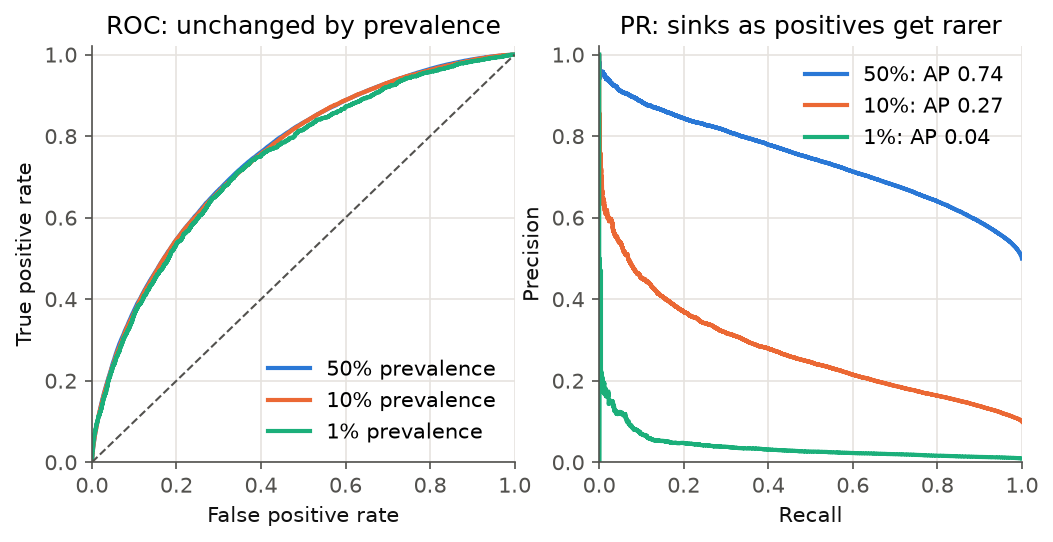
Figure 2. The same model at three prevalences. The ROC curve (left) doesn’t move. The precision–recall curve (right) collapses as positives become rare.
Read across the table. AUROC is effectively constant (the small dip at 1% is sampling noise: there are only about 2,000 positives). Precision in the top 10% falls from 86% to 3%, the difference between “most calls are useful” and “almost none are”. A model with “good” AUROC can still be operationally poor when the outcome is rare.
“AUROC asks whether the queue is in the right order. It never asks how many of the people at the front are worth calling.”
4.4 Same AUROC, different models
AUROC averages over every threshold equally, including thresholds you would never use (flagging 90% of patients). Two ROC curves can cross and still enclose the same area.
Experiment 2: equal AUROC, unequal top. Model A is the binormal model above. Model B gives positives a wider spread (σ = 1.5, mean shifted to keep the AUROC at 0.75). It’s very confident about some positives and lost on the rest. Prevalence is 10%:
| AUROC | Precision@1% | Precision@5% | Precision@30% | |
|---|---|---|---|---|
| Model A | 0.753 | 0.53 | 0.39 | 0.21 |
| Model B | 0.749 | 0.94 | 0.61 | 0.22 |
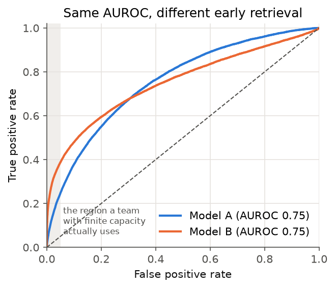
Figure 3. Two models with the same AUROC. Model B is far better in the shaded region (FPR below 5%), which is where a team with limited capacity operates. Model A wins only at thresholds nobody uses.
“A tie on the leaderboard is not a tie on the ward.”
A booking team that can call 1% of patients finds missed appointments at 94% precision with Model B and 53% with Model A, from models that a leaderboard sorted by AUROC would call tied. When only the top of the ranking matters, also report precision@k (section 6) or partial AUROC restricted to a clinically relevant FPR range.
4.5 AUROC is an estimate, so report its uncertainty
Experiment 3: how wide is the confidence interval? Same binormal model, 10% prevalence, 1,000 bootstrap resamples:
| Rows | Positives | AUROC | 95% bootstrap CI | Width |
|---|---|---|---|---|
| 600 | 66 | 0.745 | 0.680–0.807 | 0.127 |
| 6,000 | 609 | 0.752 | 0.729–0.772 | 0.043 |
| 60,000 | 5,976 | 0.751 | 0.744–0.757 | 0.013 |
The width depends mostly on the number of positives, not rows. With 66 positive cases, “AUROC 0.75” is compatible with anything from a weak model (0.68) to a strong one (0.81). Practical rules:
- Always quote a confidence interval. Use a bootstrap, or DeLong’s method (DeLong et al., 1988), which also gives a paired test for comparing two models on the same test set.
- Bootstrap whole patients, not rows, when patients repeat. Repeat appointments are correlated, so a row bootstrap makes the interval too narrow.
- A difference of 0.01–0.02 in AUROC between models is rarely meaningful on healthcare-sized data. Check the paired test before declaring a winner.
4.6 Reading AUROC values
| AUROC | Practical reading |
|---|---|
| 0.50 | No ranking information |
| 0.60–0.70 | Weak, but can still focus effort usefully (see precision@k) |
| 0.70–0.80 | Typical of good real-world models of human behaviour; published NHS outpatient DNA models sit at about 0.71–0.77 |
| 0.80–0.90 | Strong. On behavioural outcomes, audit for leakage first |
| > 0.90 | Rare for messy human outcomes. Assume a bug until proven otherwise |
The thresholds depend on context. A 0.70 on a hard problem can be more useful than a 0.90 that leaks the label.
5. Precision–recall and the prevalence baseline
The precision–recall (PR) curve plots precision against recall as the threshold moves. Unlike ROC, both of its axes are about the positive class, so it responds directly to how rare that class is (Saito & Rehmsmeier, 2015).
The usual summary is average precision (AP). Walk down the ranked list, and every time you reach a true positive, record the precision at that point. Then average those values over all positives:
- Rank 1 is a hit → 1/1 = 1.00.
- Rank 3 is a hit → 2/3 = 0.67.
- Rank 6 is a hit → 3/6 = 0.50.
- AP = 0.72.
Three things to know:
- The no-skill baseline is the prevalence, not 0.5. A random ranking has expected AP equal to the positive rate. Always quote AP next to its baseline, or as a ratio (the “AP ÷ prevalence” column in Experiment 1).
- Use the step-wise AP, not a trapezoid under the PR curve. Linear interpolation
between PR points is over-optimistic (Davis & Goadrich, 2006).
sklearn.metrics.average_precision_scoreuses the correct step-wise sum. - Name the class. AP for the majority class is near 1 by construction. In my hackathon notebook, “AP 0.94” turned out to be for the attended class, whose baseline was 0.91.
6. Precision@k: the metric for teams with finite capacity
A team with twenty phone slots is like a lifeboat with twenty seats. What matters is who is in the boat, not how well the whole queue on the deck was ordered. If a team can act on k cases per period, only the top k of the ranking matter:
def precision_at_k(y_true, scores, k):
    """Share of true positives among the k highest-scoring cases."""
    top_k = np.argsort(-scores)[:k]
    return y_true[top_k].mean()

def recall_at_k(y_true, scores, k):
    """Share of all positives that land in the top k."""
    top_k = np.argsort(-scores)[:k]
    return y_true[top_k].sum() / y_true.sum()
Lift@k is precision@k divided by prevalence: how many times better than calling at random. In the hackathon model, the top 10% by risk had a 16.3% missed rate against an 8.8% baseline (lift ≈ 1.9×), and held 19.5% of all missed appointments. “Each call is about twice as likely to reach someone who would have missed” is a sentence a service manager can act on. “AUROC 0.62” isn’t.
Two cautions:
- Fix k before you look at the test set. Choosing k after seeing the results is a quiet form of overfitting.
- Simulate the real cadence. If scoring runs weekly, compute precision@k for each week and report the distribution, not one pooled figure.
7. Calibration: can you read the score as a probability?
Think of a weather forecaster. On all the days she says “70% chance of rain”, it should rain on about 70% of them. If it rains on only 40%, she may still be excellent at telling wet days from dry ones (good ranking), but you can’t plan a picnic on her numbers (poor calibration).
A model is calibrated in the same sense: among cases scored at 0.2, about 20% are positive. AUROC can’t see this (property 1 in section 4.3), so it needs its own checks.
“Ranking well and telling the truth about probabilities are two different skills.”
Experiment 4: distort the probabilities, watch AUROC stay still.
- I fitted a logistic regression on simulated data with 10% prevalence.
- I distorted its output by doubling the logit and shifting it. This is a monotone change, so the ranking is untouched, but the model becomes over-confident.
- I repaired the distorted output with isotonic regression, fitted on a separate calibration split.
| Model | AUROC | Brier | Calibration slope | Calibration intercept |
|---|---|---|---|---|
| Well specified | 0.780 | 0.0817 | 0.98 | −0.09 |
| Distorted (monotone) | 0.780 | 0.0885 | 0.49 | −0.83 |
| Isotonic-recalibrated | 0.779 | 0.0819 | 0.95 | −0.10 |
| Always predict prevalence | 0.500 | 0.0930 | — | — |
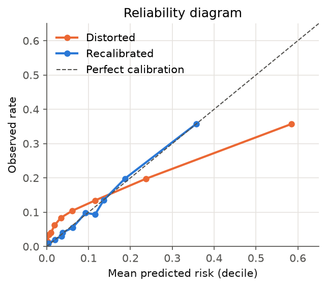
Figure 4. Reliability diagram: ten equal-sized groups by predicted risk. The distorted model’s top group predicts 58% but only 36% occur. Recalibration puts the points back on the diagonal without changing the ranking.
How to read the summaries:
- Calibration slope is the coefficient from regressing the outcome on the model’s
logit.
- 1 is ideal.
- Below 1 means predictions are too extreme. This is the usual sign of overfitting.
- Above 1 means predictions are too timid.
- Calibration intercept (calibration-in-the-large) checks whether predictions are too high or too low on average.
- Brier score is the mean of (p − y)². It combines calibration and discrimination, so compare it with the “always predict prevalence” reference (0.0930 here) rather than reading it on its own.
- Reliability diagram: plot it. A single number hides where the miscalibration is.
Real data shows the same problem. My hackathon model’s “very high” risk group predicted 34.6% and observed 20.3%. Van Calster et al. (2019) call calibration “the Achilles heel of predictive analytics” for exactly this reason: models get validated on AUROC and deployed showing percentages.
Recalibration options:
- Platt scaling fits a logistic regression on the logit. It’s best for small data.
- Isotonic regression is flexible and monotone. It needs more data.
Both must be fitted on data not used to train the model. Also note that resampling tricks (SMOTE, undersampling) and class weights deliberately shift predicted probabilities. If you use them, recalibrate afterwards.
8. Net benefit: is the model worth using at all?
None of the metrics so far answers the question a service owner actually asks: is acting on this model better than the simple alternatives? Decision curve analysis (Vickers & Elkin, 2006) does.
For a threshold probability pₜ:
Net benefit = TP / N − (FP / N) × pₜ / (1 − pₜ)
The factor pₜ / (1 − pₜ) is an exchange rate. Choosing pₜ = 0.10 says “I’d accept 9 unnecessary calls to prevent one missed appointment”. It works like an insurance premium: how much unnecessary effort you’re willing to pay to prevent one bad outcome. The model is compared with two defaults: call everyone and call no one (net benefit 0).
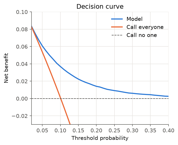
Figure 5. Decision curve for the 10%-prevalence binormal model, recalibrated to probabilities.
| Threshold pₜ | Model | Call everyone | Reading |
|---|---|---|---|
| 0.05 | 0.061 | 0.054 | The model adds a little over calling everyone |
| 0.10 | 0.037 | 0.001 | Calling everyone is worth nothing at this exchange rate; the model still helps |
| 0.20 | 0.014 | −0.124 | Calling everyone does net harm; the model remains positive |
Net benefit is measured in “true positives per patient, after charging for false positives”. A net benefit of 0.037 means the equivalent of 3.7 missed appointments correctly targeted per 100 patients, at no false-positive cost. If a model’s curve dips below “call everyone” or “call no one” across the plausible range of pₜ, it shouldn’t be deployed, however good its AUROC.
9. Beyond AUROC: more metrics worth knowing
The metrics above cover most risk-model reviews. These are the others you will meet in papers, vendor reports and model cards, with the worked-example value where one applies (threshold 0.5: TP 2, FP 2, FN 1, TN 5):
Threshold metrics that cope with imbalance
| Metric | Formula / idea | Worked example | When it helps | Watch out for |
|---|---|---|---|---|
| Balanced accuracy | (recall + specificity) / 2 | 0.69 | A quick fix for the “accuracy on rare outcomes” trap; 0.5 = chance | Still hides the precision cost |
| Matthews correlation coefficient (MCC) | (TP·TN − FP·FN) / √[(TP+FP)(TP+FN)(TN+FP)(TN+FN)] | 0.36 | One threshold number that uses all four cells; −1 to +1, 0 = chance | Hard to explain to non-specialists |
| Cohen’s kappa | (observed agreement − chance agreement) / (1 − chance agreement) | 0.35 | Agreement beyond chance, e.g. model vs human coder | Depends on prevalence; can be low even when agreement looks high |
| F-beta (F2, F0.5) | Weighted harmonic mean; β > 1 favours recall | F2 0.63 · F0.5 0.53 | When missing a positive costs more (F2) or less (F0.5) than a false alarm | The weight should come from real costs, not habit |
| Negative predictive value (NPV) | TN / (TN + FN) | 0.83 | “If the model says attend, how sure can we be?” — key for rule-out tools | Depends on prevalence, like precision |
| Youden’s J | recall + specificity − 1 | 0.38 | Picks a threshold that balances the two error rates | Assumes both errors cost the same, which they rarely do |
Ranking and threshold-free metrics
| Metric | What it measures | Worked example | Note |
|---|---|---|---|
| Kolmogorov–Smirnov (KS) | Largest gap between TPR and FPR over all thresholds | 0.57 | Common in credit scoring; it’s the tallest vertical gap between the ROC curve and the diagonal |
| Partial AUROC | Area under the ROC curve within a chosen FPR range (e.g. 0–5%) | — | Focuses on the region a capacity-limited team uses (section 4.4) |
| Sensitivity at fixed specificity | Recall when specificity is held at, say, 95% | — | Common in screening studies; easy to explain |
| NDCG@k, MRR, hit@k | How high the right answers appear in a ranked list | — | The language of search and recommendation; NDCG@5/@10 scored my SMART 2021 answer-type system |
Probability and calibration metrics
| Metric | What it measures | Worked example | Note |
|---|---|---|---|
| Log loss (cross-entropy) | Average −log(probability given to the true outcome) | 0.52 (vs 0.61 for always predicting 0.3) | Punishes confident wrong answers hard; the loss most models are trained on |
| Expected calibration error (ECE) | Weighted average gap between predicted and observed rates across bins | 0.20 (5 bins) | Popular in ML papers, but sensitive to the binning choice; prefer a plot plus slope and intercept |
Operational metrics
| Metric | What it measures | Note |
|---|---|---|
| Number needed to alert (NNA) | 1 / precision@k: actions per true positive found | In the worked example the top 3 contain 2 positives, so NNA@3 = 1.5 calls per missed appointment |
| Number needed to treat (NNT) | 1 / absolute risk reduction from the intervention | Not a model metric, but it turns model output into effort: precision tells you who to call, NNT tells you how many calls prevent one miss |
| Alert rate | Share of cases flagged per period | The first number an operations lead asks for; must fit capacity |
For forecasts and continuous predictions
Not every model in a portfolio is a classifier. For projections and regressions:
| Metric | What it measures | Note |
|---|---|---|
| MAE | Average absolute error, in the outcome’s own units | The easiest to explain |
| RMSE | Square root of average squared error | Penalises large misses more than MAE |
| MAPE / sMAPE | Average percentage error | Unstable when actual values are near zero |
| Prediction-interval coverage | Share of actual values that fall inside the stated interval | A “95%” band that covers 70% of outcomes is a calibration failure |
| Backtest (rolling origin) | Fit on data up to time t, forecast t+h, repeat | The forecasting equivalent of a temporal split |
“More metrics don’t make a better evaluation. Choose the few that answer the questions your users ask, and report their baselines.”
10. What to report, and common traps
Matching questions to metrics
| Question | Metric |
|---|---|
| Does the model rank cases better than chance? | AUROC with a 95% CI (bootstrap or DeLong) |
| How much better than chance on a rare outcome? | AP with its prevalence baseline |
| How well does acting on the top k work? | Precision@k, recall@k, lift@k, per scoring cycle |
| Can the score be read as a probability? | Calibration slope and intercept, reliability diagram, Brier score |
| What are the error trade-offs at this threshold? | Confusion matrix, precision, recall, specificity |
| Is acting on it better than simple defaults? | Decision curve / net benefit |
| Does it work for everyone? | All of the above, by subgroup |
For clinical prediction models, the TRIPOD+AI reporting guideline (Collins et al., 2024) turns this into a checklist, including fairness items.
Traps I’ve seen, or fallen into
- Not naming the positive class. “Precision 0.94” is meaningless until you know whether it’s for “missed” or “attended”.
- Quoting a metric without its baseline. That means 0.5 for AUROC, the prevalence for AP, and the majority-class rate for accuracy.
- Choosing the threshold on the test set. Tune on validation data, then report on untouched test data.
- Random splits on data that has time order or repeat patients. These inflate every metric above. Split by time, and group by patient.
- Comparing models that differ by 0.01 in AUROC without a paired test.
- Showing uncalibrated scores as percentages to people who will act on them.
- Celebrating a suspiciously high AUROC. On noisy human outcomes, 0.90 more often means leakage, such as a feature recorded after the outcome, than a breakthrough.
11. Three questions before you trust a risk model
Back to the service manager’s question. Before any model goes in front of a team, it should be able to answer three questions, in this order:
First, does it rank? Is the AUROC clearly above 0.5, with a confidence interval that excludes “weak”, on a validation set that mimics deployment (split by time, grouped by patient)? If not, stop here.
Second, does it work where we act? At the team’s real capacity, what are precision@k and lift? This is the honest answer to “how many of the twenty would have missed?” A model that ranks well on average but poorly at the top is the wrong model for a team with twenty slots.
Third, can its numbers be believed, and is acting on them worth it? Is it calibrated, so a “20%” on screen means 20%? Does the decision curve stay above “call everyone” and “call no one” across the exchange rates the service would accept? And do all three answers hold for every patient group, not just on average?
“A good model isn’t the one with the highest number on the last slide. It’s the one whose numbers answer the questions the people using it actually ask.”
References
- Hanley JA, McNeil BJ (1982). The meaning and use of the area under a receiver operating characteristic (ROC) curve. Radiology 143(1).
- DeLong ER, DeLong DM, Clarke-Pearson DL (1988). Comparing the areas under two or more correlated ROC curves: a nonparametric approach. Biometrics 44(3).
- Davis J, Goadrich M (2006). The relationship between precision-recall and ROC curves. ICML.
- Saito T, Rehmsmeier M (2015). The precision-recall plot is more informative than the ROC plot when evaluating binary classifiers on imbalanced datasets. PLoS ONE.
- Vickers AJ, Elkin EB (2006). Decision curve analysis: a novel method for evaluating prediction models. Medical Decision Making.
- Van Calster B et al. (2019). Calibration: the Achilles heel of predictive analytics. BMC Medicine.
- Collins GS et al. (2024). TRIPOD+AI statement. BMJ.
Further reading on this site
-
Would my own models pass? Auditing five ML models against my evaluation checklist — this checklist applied to every ML model in my repositories.
- Predicting missed outpatient appointments: two case studies and what the evidence says — these metrics applied to a real problem.
- Accuracy matters, but usefulness matters more